ASTRE
A-contrario Smooth TRajectory Extraction
Presentation
Download / Installation and usage manual
Snow data sequence
Table of contents
Download the code
License
This program is released under GPL License.
Feel free to use and adapt this code. However, if you use it for your
research or in software code, please cite the
accompanying paper.
Also, if you use, adapt or improve the code, we would love to
hear
about it! (simply replace [AT] by @ in the e-mail address)
Download
-
Download the code (128 kB)
C source code for the trajectory detection, and Python trajectory visualizer.
Installation
Requirements
This program is released under GPL License.
Feel free to use and adapt this code. However, if you use it for your research or in software code, please cite the accompanying paper.
Also, if you use, adapt or improve the code, we would love to hear about it! (simply replace [AT] by @ in the e-mail address)
-
Download the code (128 kB)
C source code for the trajectory detection, and Python trajectory visualizer.
You need an environment providing a C compiler (tested with gcc 4.3), as well as Python and PyQt4 for the visualization tools (optional, see below for the installation)
Install the dependencies
Download and install cbase (version 1.3.5 or greater) from our local copy or from the project website :
$ tar -xzf cbase-1.3.5.tar.gz
$ cd cbase-1.3.5
$ ./configure
$ make
$ sudo make install
$ cd ..
Download and install argtable2 (version 1.3 or greater) from our local copy or from the project site :
$ tar -xzf argtable2-13.tar.gz
$ cd argtable2-13
$ ./configure
$ make
$ sudo make install
$ cd ..
Add the library installation path to the LD_LIBRARY_PATH environment variable in your .bash_profile or .profile file:
export LD_LIBRARY_PATH=/usr/local/lib:${LD_LIBRARY_PATH}
You can then remove the source directories cbase-1.3.5 and argtable2-13 that are no longer needed.
Install ASTRE
Download ASTRE and compile the binaries:
$ tar -xzf astre-1.0.tar.gz
$ cd astre-1.0
$ make
Add the Python library path to your PATH environment variable in your .bash_profile or .profile file:
export PATH=/path/to/astre-1.0/bin:${PATH}
Install the visualization tools [optional]
Install Python and PyQt4:
$ sudo apt-get install python python-qt4
Add the Python library path to your PYTHONPATH environment variable in your .bash_profile or .profile file:
export PYTHONPATH=/path/to/astre-1.0/lib/python/:${PYTHONPATH}
❦
Tutorial
Usage of ASTRE and visualization of the results
Visualize points description files
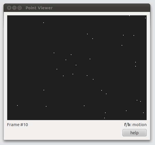
If you have installed the Python libraries, you can use the tview.py points description files viewer.
ASTRE comes bundled with sample data in the data directory. To visualize the snow sequence, type
$ tview.py data/snow.30Hz.descand press f(orward) and b(ackward) to move through the sequence.
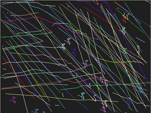
Run ASTRE on the snow sequence
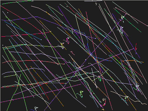
We run ASTRE (without holes) on the trajectory set and visualize the found trajectories using the -t option of tview.py with parameter log10(ε) = 0 (maximal value of log10(NFA))
$ astre-noholes -e 0.0 data/snow.30Hz.desc tjs
$ tview.py -t tjs

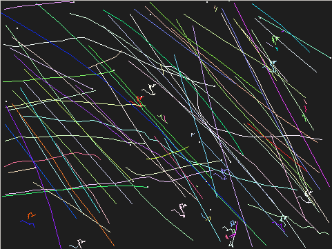
We can run ASTRE (without holes) with a larger parameter to discover more trajectories:
$ astre-noholes -e 5.0 data/snow.30Hz.desc tjs
$ tview.py -t tjs
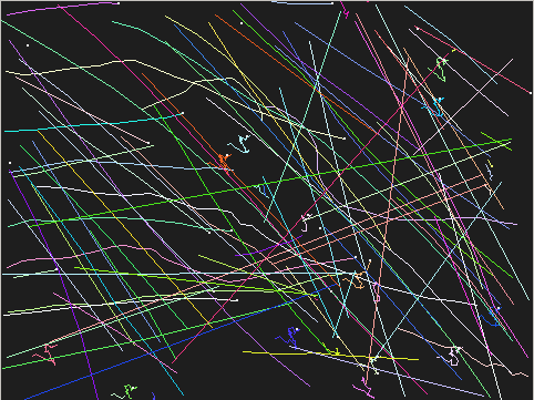
You could do the same with astre-holes to obtain the results shown in our paper, but this takes much more time and memory on such a large sequence. You can however use the -h parameter of astre-holes to limit the size of the holes in a trajectory, and speed up the computation at the expense of finding suboptimal solutions (the computation took about 2 minutes on a standard laptop):
$ astre-holes -e 5.0 -h 1 data/snow.30Hz.desc tjs
$ tview.py -t tjs
As a reference, this is the computation times on a standard laptop for astre-holes with parameter log10(ε) = 0 and various values of the h parameter on the snow sequence (which has 40 frames):
| h | 1 | 2 | 3 | 4 | 5 | 10 | 20 | 30 | 40 |
| time | 1 min | 4 min | 6 min | 10 min | 12 min | 23 min | 33 min | 34 min | 35 min |
astre-noholes and astre-holes copy the input points description file to the output and add a column containing the trajectory identifier (or -1 if the point does not belong to a trajectory).
Note also that astre-noholes and astre-holes add a header for each detected trajectory of the form traj:<id>:lNFA = <lNFA> showing the log10 NFA of the corresponding trajectory id.
Evaluation of ASTRE results
Algorithm evaluation on real data
A qualitative visual inspection of the found trajectories already gives a rough idea of the algorithms performances. Yet one would sometimes rather have a way to quantify those performances.
The recall and the precision of the detections can be computed using the tstats program. Rather than taking into account only whole trajectories (without any missing or spurious point), we chose to compute the recall and precision in terms of the number of correct links found, that is, two consecutive points on a trajectory, possibly separated by a hole. The recall and precision are then:
precision = # of correct links / # of found links
where a link is real if it belongs to the ground-truth, is found if it belongs to the detected trajectories and is correct if it belongs to both.
The sample snow sequence has been originally acquired at 210Hz to make it possible to reconstruct the ground-truth by hand on this simple to track version, and has then been subsampled to 30Hz to obtain a more challenging to track sequence. The snow sequence thus also contains the ground-truth, making it possible to compute the recall and precision of our results:
$ astre-noholes -e 0.0 data/snow.30Hz.desc tjs
$ tstats tjs
[MD] {'recall': 0.497377, 'precision': 0.993711,
      'num_detected_trajs': 39, }
The tstats program expects to be given a points description file with the ground truth as the fourth column and the found trajectories as the last column, but you can also specify the index of the column if needed, and even specify two different input files, one containing the ground truth, the other containing the detected trajectories.
The output array of tstats is in Python format, and the results of the experiments can be quickly processed by filtering the lines starting with [MD] (stands for metadata) and evaluating the following data structure in Python.
>>> statistics = eval("{'recall': 0.497377,
   'precision': 0.993711, 'num_detected_trajs': 39, }")
We compare the performances of astre-noholes when we increase the maximal value of the log10 NFA:
$ astre-noholes -e 5.0 data/snow.30Hz.desc tjs
$ tstats tjs
[MD] {'recall': 0.709339, 'precision': 0.948107,
      'num_detected_trajs': 124, }
Obviously, the number of detected trajectories (and thus the recall) has increased, while the precision has slightly decreased (we made some false detections).
We can now compare this last result with those of astre-holes with parameter log10(ε) = 5, both when we constrain the maximal size of a hole to 1 and when it is unbounded:
$ astre-holes -e 5.0 -h 1 data/snow.30Hz.desc tjs
$ tstats tjs
[MD] {'recall': 0.751312, 'precision': 0.939633,
      'num_detected_trajs': 99, }
Since you might not want to run the computation in the unbounded case on your computer, you might want to download the results of ASTRE on the snow sequence and compute its performances. In this case, since lNFA_5.tjs does not contain both the ground truth and the detected trajectories, but only the latter, we specify both the ground truth file and the detected trajectories file:
$ tstats snow.30Hz.desc lNFA_5.tjs
[MD] {'recall': 0.757608, 'precision': 0.916244,
      'num_detected_trajs': 91, }
Clearly, we have gained almost nothing in recall, but slightly lost in precision by allowing unbounded hole lengths. However, this might be due to properties of this particular data and might not be the case in a more general setting.
As a reference, here is a table with the recall, precision and number of detected trajectories for astre-holes on the snow sequence with parameter log10(ε) = 0 and various values for the maximal hole length parameter h (the sequence spans 40 frames):
| h | 1 | 2 | 3-6 | 7-40 |
| recall | 0.54 | 0.54 | 0.54 | 0.55 |
| prec. | 0.94 | 0.93 | 0.92 | 0.91 |
| #trajs | 36 | 35 | 33 | 34 |
and when log10(ε) = 5
| h | 1 | 2 | 3-6 | 7-40 |
| recall | 0.75 | 0.76 | 0.76 | 0.76 |
| prec. | 0.94 | 0.93 | 0.92 | 0.92 |
| #trajs | 99 | 94 | 93 | 91 |
Systematic algorithm evaluation using synthetic trajectories
We generate 5 trajectories spanning 20 frames, add 10 random noise points in each frame and then remove 20% of the trajectory points, and run ASTRE (with holes) with the default parameter log10(ε) = 0:
$ tpsmg -N 10 20 5 pts
$ tcripple -r 20 pts pts
$ astre-holes pts tjs
Note that when generating (integer-valued) point description files with tpsmg, we forbid two trajectories from sharing a point (otherwise the overlapping trajectory is regenerated), and we do not add noise points at the same location as one trajectory point. By default, all trajectories are constrained to stay in the frame (otherwise they are regenerated), but this behavior can be changed with the -F option (see below for a description of the astre options).
Also note that when crippling points description files with tcripple, only points belonging to a trajectory are removed (the noise points are kept).
❦
ASTRE points and trajectories data file format
The format of the files is the following
type = PointsFile v.1.0
uid = 1
width = 480
height = 360
DATA
0 292 204 4
0 247 304 51
...
All the lines before DATA are headers of the form key = value, and all the lines after DATA are array of floats representing one point, the minimum data for a point is 3 column:
<frame> <x> <y>
but often they have a trajectory identifier
<frame> <x> <y> <t>where t is the id of the trajectory to which the point belong, or -1 if the point does not belong to a trajectory.
The data entries can be preceded by an optional column name:
f:0 x:292 y:204 t:4
...
in which case, all the tags of one column must be the same.
If you need it, you can add other data columns to represent the intensity of the points, etc. It is also possible to add length-varying descriptors (for instance, a polygonal shape descriptor) by using special headers: describe each shape with a unique identifier as header entries, and reference the corresponding identifier in your data column:
type = PointsFile v.1.0
...
shape:0 = (4.0, 18.0) (17.0, 10.0) ... (14.0, 18.0)
shape:1 = (2.0, 5.0) (14.0, 11.0) ... (5.0, 15.0)
...
DATA
<frame> <x> <y> <shape_id> <trajectory_id>
...
The required headers are
- type to identify the file format version (its value should be PointsFile v.1.0),
- width and height representing the frame size,
- uid with an integer identifier representing the data. This can be an arbitrary integer, and from our personal experience, it sometimes proves useful to avoid accidentally mixing data and this is why it is mandatory, although you can safely set it to 0 if you do not plan to use it.
❦
User reference
astre-holes
ASTRE (astre-noholes and astre-holes)
The astre-noholes and astre-holes programs greedily detect trajectories in a points description file using the a-contrario framework. The astre-noholes can be used when the trajectories do not contain holes, and its detection criterion is optimized for this case. In general, astre-noholes is faster and more memory-efficient than astre-holes.
The basic usage to detect trajectories of log10 NFA less than 0 is:
$ astre-noholes <in> <out>
$ astre-holes <in> <out>
The options are:
|
--epsilon <e> (or -e <e>) |
set the maximal log10 NFA for the trajectories detection Warning: -e 0.0 (default) means log10(ε)=0, that is, ε=1 |
| --max-hole-length <h> (or -h <h>) | set the maximal size of a hole when using astre-noholes (default: any length). This can be used to lower the computational and memory costs, at the expense of not considering all the possible trajectories. |
ASTRE adds a column containing trajectory identifiers, or -1 if a point does not belong to a detected trajectory. It also adds headers of the form traj:<id>:lNFA = <lNFA> that describe the log10 NFA of each trajectory.
Using the programs with the option --tag-NFA only tags each trajectory with its NFA and exits. This can be useful if you have detected trajectories using another program, and want to filter out trajectories above a certain NFA.
For long computations, you might want ASTRE to periodically save the partial detections, to make detection backups or to monitor detected trajectories. This is possible using the --save-partial <filename> option. Restarting a computation is done using the --restart option and using the partial detections file as input:
$ astre-holes --save-partial partial_tjs pts tjs
...[interrupt computations]
$ astre-holes --save-partial partial_tjs --restart partial_tjs tjs
Finally, the auto-crop option is not thoroughly tested but might help detecting trajectories when image sequences have some points in the center of the images and a lot of empty space around, by automatically cropping the empty space, which changes the implicit scale of the images, and hence the NFA.
Recall and precision computation (tstats)
The tstats program outputs the recall and precision defined in terms of real, correct and found links, as well as the number of detected trajectories.
The basic usage is:
$ tstats [<ground truth file>] <detected trajectories file>
If the ground truth file is not specified, this assumes that the detected trajectories file contains both the ground truth and the trajectories detected by the algorithm. The ground truth and the detected trajectories file must have the same uid header. By default, the ground truth file should have the trajectories identifiers in the fourth column and the detected trajectories file should have them in the last column.
A link is two successive (possibly separated by a hole) detected points in a trajectory. A link is real if it belongs to the ground truth, it is found if it belongs to the detected trajectories, and it is correct if it belongs to both.
The recall is # correct links / # real links and the precision is # correct links / # found links. The recall corresponds to the proportion of real points that have been detected, while the precision corresponds to the proportion of detected points that are correct, that is, it inversely relates to the number of false detections.
The options are:
|
--real-traj <r> (or -r <r>) |
the 0-based index of the column containing the real trajectories in the ground truth points description file (default: 3) |
|
--found-traj <f> (or -f <f>) |
the 0-based index of the column containing the real trajectories in the detected trajectories points description file (default: -1, the last column) |
PSMG Point Set Motion Generator (tpsmg)
The tpsmg program emulates the Point Set Motion Generator, that randomly draws some points in the image frame and displace them by updating their acceleration from frame to frame with a gaussian variable.
The basic usage to generate n trajectories spanning K frames in the file out is:
$ tpsmg <K> <n> <out>
The options are:
| -N <N> | add N noise points to each image (the noise points cannot share the location of a trajectory point) |
| -r | the number of noise points added to each image is not constant, but rather a number drawn uniformly between 0 and N |
| -F | do not force trajectories to stay inside the frames |
| -w <w> -h <h> | set the image width and height |
| -a <a> | set the variance of the speed amplitude update (default: 0.2) |
| -o <o> | set the variance of the speed orientation update (default: 0.2) |
| -v <v> | set the mean initial speed of the trajectories (default: 5.0) |
| -V <V> | set the variance of the initial speed of the trajectories (default: 0.5) |
The trajectories are generated in the following way:
- the first point of each of the n trajectories is drawn uniformly in the first frame of the sequence,
-
each trajectory is generated in turn:
- we draw a normal variable of mean v and variance V that defines the initial speed amplitude, and a variable drawn in [0, 2π] that defines the initial speed orientation,
- we update the trajectory position according to the speed,
- we add the point to the trajectory, unless it leaves the frame or it is on the location of a previously generated trajectory, in which case we regenerate the whole trajectory,
- we draw a normal variable of mean 0 and variance a representing the speed amplitude update, and a normal variable of mean 0 and variance o representing the speed orientation update,
- we update the speed amplitude and orientation
- we add N random points in each frame such that they do not share position with a trajectory point (if the -r option is set, we add a number of noise points drawn uniformly between 0 and N,
- we shuffle the position of all the points in each frame in the points description file.
If the -F option has been set, the trajectories are not forced to stay inside the frame, and as they leave the image they are ended and a new trajectory is started in the next frame by choosing a random point uniformly on the border of the image frame and iterating the trajectory generation process. Note in this case that if a trajectory has less than 3 points in the image frame, we regenerate it, and if a trajectory leaves the image frame less than 3 frames before the end of the sequence, no new trajectory is generated, since it could not comply with the above 3-frames constraint.
Note that for some parameters, it is possible that the tpsmg does not terminate, in particular if the amplitude of the trajectory acceleration is too high, it is possible that no trajectory fits in the frame, and the program keeps trying to regenerate them.
The tpsmg program also outputs metadata indicating the global maximal speed and acceleration of the generated trajectories:
$ tpsmg 20 5 pts
[MD] { 'max_speed': 5.83095, 'max_accel': 2.82843 }
Point set crippling (tcripple)
The tcripple program remove a certain amount of points from the trajectories contained in a points description file to simulate missing detections.
Note that the number of points removed is generally not a fixed proportion of the input points, but rather, each point from a trajectory is removed with a certain probability r.
Note also that tcripple only affects point on a trajectory, that is, points having a trajectory tag different from -1 (and thus, points description files need to have a trajectory identifier column when using tcripple).
The basic usage to remove points in trajectories with probability r is:
$ tcripple -r <r> <in> <out>
The options are:
| -r <r> | the probability that a point in a trajectory is removed |
| --traj-col <t> (or -t <t>) | the 0-based index of the column containing the trajectories (default: -1, the last column) |
Viewer (tview.py)
If you have installed the Python libraries, you can use the tview.py program to view points description files and the point trajectories.
The basic usage is
$ tview.py [-t] <points description file>The option -t indicates that we want to load the trajectories contained in the points description file, where the trajectories are defined by the last column of the points description file. Points having the same identifier as the last column are in the same trajectory, and points having the special identifier -1 do not belong to any trajectory.
The options are:
| --trajectory-column <n> | the column (index is 0-based) describing the trajectories (default is -1, the last column) |
| --show-trajectories (or -t) | load and show trajectories using the trajectory identifiers in the column trajectory-column |
| f/b | go forward or backward in the sequence |
| q | quit the program |
| +/-/= | zoom in/out/default |
| t | toggle trajectory drawing (when trajectories have been loaded) |
| m | set the current frame as the first frame from which to draw trajectories |
| h | highlight the points that belong to a trajectory in red |
| x | randomize the trajectory colors |
Naive ASTRE implementation in Python (naive_astre.py)
ASTRE comes with a naive implementation in the Python language for clarity, that should however not be used with large datasets, as it is slow and requires a lot of memory.
The basic usage is
$ naive_astre.py <in> <out>and the options are
| --solver [noholes|holes] | the solver (without holes or with holes) |
| --eps <e> (or -e <e>) | the maximal value of log10(NFA) |